Hence \( T_n^2 \) is negatively biased and on average underestimates \(\sigma^2\). Estimating the mean and variance of a distribution are the simplest applications of the method of moments. This alternative approach sometimes leads to easier equations. For \( n \in \N_+ \), \( \bs X_n = (X_1, X_2, \ldots, X_n) \) is a random sample of size \( n \) from the distribution. The mean of the distribution is \(\mu = 1 / p\). If \(b\) is known then the method of moment equation for \(U_b\) as an estimator of \(a\) is \(b U_b \big/ (U_b - 1) = M\). In the reliability example (1), we might typically know \( N \) and would be interested in estimating \( r \). The method of moments estimator of \( k \) is \[ U_p = \frac{p}{1 - p} M \]. As above, let \( \bs{X} = (X_1, X_2, \ldots, X_n) \) be the observed variables in the hypergeometric model with parameters \( N \) and \( r \). Let D be the duration in hours of a battery chosen at random from the lot of production. A normal distribution is determined by two parameters the mean and the variance. Accessibility StatementFor more information contact us atinfo@libretexts.orgor check out our status page at https://status.libretexts.org. The parameter \( N \), the population size, is a positive integer. The further price action moves from the mean, in this case, the greater the likelihood that an asset is being over or undervalued. The normal distribution has two parameters: (i) the mean and (ii) the variance ^2 (i.e., the square of the standard deviation ). By clicking Accept All Cookies, you agree to the storing of cookies on your device to enhance site navigation, analyze site usage, and assist in our marketing efforts. It is the mean, median, and mode, since the distribution is symmetrical about the mean. As with our previous examples, the method of moments estimators are complicatd nonlinear functions of \(M\) and \(M^{(2)}\), so computing the bias and mean square error of the estimator is difficult. Next, \(\E(V_a) = \frac{a - 1}{a} \E(M) = \frac{a - 1}{a} \frac{a b}{a - 1} = b\) so \(V_a\) is unbiased. The average height is found to be roughly 175 cm (5' 9"), counting both males and females. WebParameters The location parameter, , is the mean of the distribution. Let us know if you have suggestions to improve this article (requires login). Solving gives the result. For example, 68.25% of all cases fall within +/- one standard deviation from the mean. Parameters of Normal Distribution 1. WebNormal distributions have the following features: symmetric bell shape mean and median are equal; both located at the center of the distribution \approx68\% 68% of the data falls within 1 1 standard deviation of the mean \approx95\% 95% of the data falls within 2 2 standard deviations of the mean \approx99.7\% 99.7% of the data falls within Kurtosis measures the thickness of the tail ends of a distribution in relation to the tails of a distribution. These include white papers, government data, original reporting, and interviews with industry experts. Note the empirical bias and mean square error of the estimators \(U\), \(V\), \(U_b\), and \(V_k\). The term Gaussian distribution refers to the German mathematician Carl Friedrich Gauss, who first developed a two-parameter exponential function in 1809 in connection with studies of astronomical observation errors. In the unlikely event that \( \mu \) is known, but \( \sigma^2 \) unknown, then the method of moments estimator of \( \sigma \) is \( W = \sqrt{W^2} \). \( \E(U_p) = k \) so \( U_p \) is unbiased. As before, the method of moments estimator of the distribution mean \(\mu\) is the sample mean \(M_n\). A basic example of flipping a coin ten times would have the number of experiments equal to 10 and the probability of However, matching the second distribution moment to the second sample moment leads to the equation \[ \frac{U + 1}{2 (2 U + 1)} = M^{(2)} \] Solving gives the result. The shape of the distribution changes as the parameter values change. What Is T-Distribution in Probability? Next, let \[ M^{(j)}(\bs{X}) = \frac{1}{n} \sum_{i=1}^n X_i^j, \quad j \in \N_+ \] so that \(M^{(j)}(\bs{X})\) is the \(j\)th sample moment about 0. Matching the distribution mean to the sample mean leads to the equation \( a + \frac{1}{2} V_a = M \). We also acknowledge previous National Science Foundation support under grant numbers 1246120, 1525057, and 1413739. 95% of all cases fall within +/- two standard deviations from the mean, while 99% of all cases fall within +/- three standard deviations from the mean. This is also known as a z distribution. The beta distribution with left parameter \(a \in (0, \infty) \) and right parameter \(b \in (0, \infty)\) is a continuous distribution on \( (0, 1) \) with probability density function \( g \) given by \[ g(x) = \frac{1}{B(a, b)} x^{a-1} (1 - x)^{b-1}, \quad 0 \lt x \lt 1 \] The beta probability density function has a variety of shapes, and so this distribution is widely used to model various types of random variables that take values in bounded intervals. Of course we know that in general (regardless of the underlying distribution), \( W^2 \) is an unbiased estimator of \( \sigma^2 \) and so \( W \) is negatively biased as an estimator of \( \sigma \). 1. = the standard deviation. As the parameter value changes, the shape of the distribution changes. Distributions with larger kurtosis greater than 3.0 exhibit tail data exceeding the tails of the normal distribution (e.g., five or more standard deviations from the mean). Although the normal distribution is an extremely important statistical concept, its applications in finance can be limited because financial phenomenasuch as expected stock-market returnsdo not fall neatly within a normal distribution. It can be used to describe the distribution of variables measured as ratios or intervals. Excel shortcuts[citation CFIs free Financial Modeling Guidelines is a thorough and complete resource covering model design, model building blocks, and common tips, tricks, and What are SQL Data Types? \( \E(U_h) = a \) so \( U_h \) is unbiased. With the help of these parameters, we can decide the shape and probabilities of the distribution wrt our problem statement. It determines how far away from the mean the data points are positioned and represents the distance between the mean and the observations. There are two main parameters of a normal distribution- the mean and standard deviation. Solving gives \[ W = \frac{\sigma}{\sqrt{n}} U \] From the formulas for the mean and variance of the chi distribution we have \begin{align*} \E(W) & = \frac{\sigma}{\sqrt{n}} \E(U) = \frac{\sigma}{\sqrt{n}} \sqrt{2} \frac{\Gamma[(n + 1) / 2)}{\Gamma(n / 2)} = \sigma a_n \\ \var(W) & = \frac{\sigma^2}{n} \var(U) = \frac{\sigma^2}{n}\left\{n - [\E(U)]^2\right\} = \sigma^2\left(1 - a_n^2\right) \end{align*}. 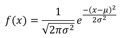 The standard normal distribution is a probability distribution, so the area under the curve between two points tells you the probability of variables taking on a range of values. Suppose that \(b\) is unknown, but \(k\) is known. The normal distribution has two parameters, the mean and standard deviation. Solving gives (a). The normal distribution follows the following formula. Financial Modeling & Valuation Analyst (FMVA), Commercial Banking & Credit Analyst (CBCA), Capital Markets & Securities Analyst (CMSA), Certified Business Intelligence & Data Analyst (BIDA), Financial Planning & Wealth Management (FPWM). WebA z-score is measured in units of the standard deviation.
  \(\var(V_a) = \frac{b^2}{n a (a - 2)}\) so \(V_a\) is consistent. Suppose that \( a \) and \( h \) are both unknown, and let \( U \) and \( V \) denote the corresponding method of moments estimators. x = value of the variable or data being examined and f (x) the probability function. Standard Deviation So any of the method of moments equations would lead to the sample mean \( M \) as the estimator of \( p \). Equivalently, \(M^{(j)}(\bs{X})\) is the sample mean for the random sample \(\left(X_1^j, X_2^j, \ldots, X_n^j\right)\) from the distribution of \(X^j\). Corrections? Probability Density Function (PDF) When one of the parameters is known, the method of moments estimator of the other parameter is much simpler. Our editors will review what youve submitted and determine whether to revise the article. Suppose that the mean \(\mu\) is unknown. The two parameters for the Binomial distribution are the number of experiments and the probability of success. Then \[ U_b = b \frac{M}{1 - M} \]. Then \[U = \frac{M \left(M - M^{(2)}\right)}{M^{(2)} - M^2}, \quad V = \frac{(1 - M)\left(M - M^{(2)}\right)}{M^{(2)} - M^2}\]. The mean is used by researchers as a measure of central tendency. Of course, the method of moments estimators depend on the sample size \( n \in \N_+ \). Note that the mean \( \mu \) of the symmetric distribution is \( \frac{1}{2} \), independently of \( c \), and so the first equation in the method of moments is useless. Moivres theory was expanded by another French scientist, Pierre-Simon Laplace, in Analytic Theory of Probability. Laplaces work introduced the central limit theorem that proved that probabilities of independent random variables converge rapidly to the areas under an exponential function. Suppose now that \( \bs{X} = (X_1, X_2, \ldots, X_n) \) is a random sample of size \( n \) from the uniform distribution. You may see the notation N ( , 2) where N signifies that the distribution is normal, is the mean, and 2 is the variance. Run the normal estimation experiment 1000 times for several values of the sample size \(n\) and the parameters \(\mu\) and \(\sigma\). With the help of these parameters, we can decide the shape and probabilities of the distribution wrt our problem statement. In addition, \( T_n^2 = M_n^{(2)} - M_n^2 \). The resultant graph appears as bell-shaped where the mean, median, and mode are of the same values and appear at the peak of the curve. Solving for \(U_b\) gives the result. The standard normal distribution is a probability distribution, so the area under the curve between two points tells you the probability of variables taking on a range of values. This article was most recently revised and updated by, https://www.britannica.com/topic/normal-distribution, Khan Academy - Normal distributions review (article) | Khan Academy, Statistics LibreTexts - Normal Distribution. Structured Query Language (known as SQL) is a programming language used to interact with a database. Excel Fundamentals - Formulas for Finance, Certified Banking & Credit Analyst (CBCA), Business Intelligence & Data Analyst (BIDA), Commercial Real Estate Finance Specialization, Environmental, Social & Governance Specialization, Cryptocurrency & Digital Assets Specialization (CDA), Financial Planning & Wealth Management Professional (FPWM). The first two moments are \(\mu = \frac{a}{a + b}\) and \(\mu^{(2)} = \frac{a (a + 1)}{(a + b)(a + b + 1)}\). 1) Calculate 1 and 1 2 knowing that P ( D 47) = 0, 82688 and P ( D 60) = 0, 05746. The normal distribution is one type of symmetrical distribution. The mean is \(\mu = k b\) and the variance is \(\sigma^2 = k b^2\). What are the properties of normal distributions? = the mean. Suppose that \( a \) is known and \( h \) is unknown, and let \( V_a \) denote the method of moments estimator of \( h \). The calculation is as follows: x = + ( z ) ( ) = 5 + (3) (2) = 11. \( \E(V_a) = 2[\E(M) - a] = 2(a + h/2 - a) = h \), \( \var(V_a) = 4 \var(M) = \frac{h^2}{3 n} \). 11.1: Prelude to The Normal Distribution The normal, a continuous distribution, is the Legal. Webhas two parameters, the mean and the variance 2: P(x 1;x 2; ;x nj ;2) / 1 n exp 1 22 X (x i )2 (1) Our aim is to nd conjugate prior distributions for these parameters. Suppose that \( \bs{X} = (X_1, X_2, \ldots, X_n) \) is a random sample from the symmetric beta distribution, in which the left and right parameters are equal to an unknown value \( c \in (0, \infty) \). The z -score is three. Note also that, in terms of bias and mean square error, \( S \) with sample size \( n \) behaves like \( W \) with sample size \( n - 1 \). However, the distribution makes sense for general \( k \in (0, \infty) \). If \(a \gt 2\), the first two moments of the Pareto distribution are \(\mu = \frac{a b}{a - 1}\) and \(\mu^{(2)} = \frac{a b^2}{a - 2}\). It can be used to describe the distribution of 2. All normal distributions can be described by just two parameters: the mean and the standard deviation. With the help of these parameters, we can decide the shape and probabilities of the distribution wrt our problem statement. On the other hand, \(\sigma^2 = \mu^{(2)} - \mu^2\) and hence the method of moments estimator of \(\sigma^2\) is \(T_n^2 = M_n^{(2)} - M_n^2\), which simplifies to the result above. In fact, if the sampling is with replacement, the Bernoulli trials model would apply rather than the hypergeometric model. WebThis study investigates, for the first time, the product of spacing estimation of the modified Kies exponential distribution parameters as well as the acceleration factor using constant-stress partially accelerated life tests under the Type-II censoring scheme. Take, for example, the distribution of the heights of human beings. However, we can judge the quality of the estimators empirically, through simulations. With two parameters, we can derive the method of moments estimators by matching the distribution mean and variance with the sample mean and variance, rather than matching the distribution mean and second moment with the sample mean and second moment. As the parameter value changes, the shape of the distribution changes. Meanwhile, taller and shorter people exist, but with decreasing frequency in the population. This fact is sometimes referred to as the "empirical rule," a heuristic that describes where most of the data in a normal distribution will appear. A t-distribution is a type of probability function that is used for estimating population parameters for small sample sizes or unknown variances. Suppose that \(a\) and \(b\) are both unknown, and let \(U\) and \(V\) be the corresponding method of moments estimators. If \(b\) is known then the method of moments equation for \(U_b\) as an estimator of \(a\) is \(U_b \big/ (U_b + b) = M\). The geometric distribution on \( \N \) with success parameter \( p \in (0, 1) \) has probability density function \[ g(x) = p (1 - p)^x, \quad x \in \N \] This version of the geometric distribution governs the number of failures before the first success in a sequence of Bernoulli trials. The normal distribution has two parameters (two numerical descriptive measures), the mean () and the standard deviation (). Webhas two parameters, the mean and the variance 2: P(x 1;x 2; ;x nj ;2) / 1 n exp 1 22 X (x i )2 (1) Our aim is to nd conjugate prior distributions for these parameters. 2) Calculate the density function of the duration in hours for a battery chosen at random from the lot. On the other hand, in the unlikely event that \( \mu \) is known then \( W^2 \) is the method of moments estimator of \( \sigma^2 \). We sample from the distribution to produce a sequence of independent variables \( \bs X = (X_1, X_2, \ldots) \), each with the common distribution. In finance, most pricing distributions are not, however, perfectly normal. On the graph, the standard deviation determines the width of the curve, and it tightens or expands the width of the distribution along the x-axis. We also acknowledge previous National Science Foundation support under grant numbers 1246120, 1525057, and 1413739. The mean, median and mode are exactly the same. More generally, the negative binomial distribution on \( \N \) with shape parameter \( k \in (0, \infty) \) and success parameter \( p \in (0, 1) \) has probability density function \[ g(x) = \binom{x + k - 1}{k - 1} p^k (1 - p)^x, \quad x \in \N \] If \( k \) is a positive integer, then this distribution governs the number of failures before the \( k \)th success in a sequence of Bernoulli trials with success parameter \( p \). We start by estimating the mean, which is essentially trivial by this method. As usual, we get nicer results when one of the parameters is known. The parameter \( r \) is proportional to the size of the region, with the proportionality constant playing the role of the average rate at which the points are distributed in time or space. \(\mse(T^2) = \frac{2 n - 1}{n^2} \sigma^4\), \(\mse(T^2) \lt \mse(S^2)\) for \(n \in \{2, 3, \ldots, \}\), \(\mse(T^2) \lt \mse(W^2)\) for \(n \in \{2, 3, \ldots\}\), \( \var(W) = \left(1 - a_n^2\right) \sigma^2 \), \( \var(S) = \left(1 - a_{n-1}^2\right) \sigma^2 \), \( \E(T) = \sqrt{\frac{n - 1}{n}} a_{n-1} \sigma \), \( \bias(T) = \left(\sqrt{\frac{n - 1}{n}} a_{n-1} - 1\right) \sigma \), \( \var(T) = \frac{n - 1}{n} \left(1 - a_{n-1}^2 \right) \sigma^2 \), \( \mse(T) = \left(2 - \frac{1}{n} - 2 \sqrt{\frac{n-1}{n}} a_{n-1} \right) \sigma^2 \). The normal distribution with mean \( \mu \in \R \) and variance \( \sigma^2 \in (0, \infty) \) is a continuous distribution on \( \R \) with probability density function \( g \) given by \[ g(x) = \frac{1}{\sqrt{2 \pi} \sigma} \exp\left[-\frac{1}{2}\left(\frac{x - \mu}{\sigma}\right)^2\right], \quad x \in \R \] This is one of the most important distributions in probability and statistics, primarily because of the central limit theorem. The two parameters for the Binomial distribution are the number of experiments and the probability of success. WebNormal distributions have the following features: symmetric bell shape mean and median are equal; both located at the center of the distribution \approx68\% 68% of the data falls within 1 1 standard deviation of the mean \approx95\% 95% of the data falls within 2 2 standard deviations of the mean \approx99.7\% 99.7% of the data falls within Probability Density Function (PDF) The point What are the properties of normal distributions? Besides this approach, the conventional maximum likelihood method is also considered. One would think that the estimators when one of the parameters is known should work better than the corresponding estimators when both parameters are unknown; but investigate this question empirically. The method of moments works by matching the distribution mean with the sample mean. Form our general work above, we know that if \( \mu \) is unknown then the sample mean \( M \) is the method of moments estimator of \( \mu \), and if in addition, \( \sigma^2 \) is unknown then the method of moments estimator of \( \sigma^2 \) is \( T^2 \). We compared the sequence of estimators \( \bs S^2 \) with the sequence of estimators \( \bs W^2 \) in the introductory section on Estimators. Suppose that \(\bs{X} = (X_1, X_2, \ldots, X_n)\) is a random sample of size \(n\) from the geometric distribution on \( \N_+ \) with unknown success parameter \(p\). Discover your next role with the interactive map. The beta distribution is studied in more detail in the chapter on Special Distributions. The mean, median and mode are exactly the same. The calculation is as follows: x = + ( z ) ( ) = 5 + (3) (2) = 11. Thus, we will not attempt to determine the bias and mean square errors analytically, but you will have an opportunity to explore them empricially through a simulation. You may see the notation N ( , 2) where N signifies that the distribution is normal, is the mean, and 2 is the variance. Figure 1. The Pareto distribution is studied in more detail in the chapter on Special Distributions. A normal distribution is symmetric from the peak of the curve, where the mean is. = the standard deviation. A standard normal distribution (SND). In this case, the sample \( \bs{X} \) is a sequence of Bernoulli trials, and \( M \) has a scaled version of the binomial distribution with parameters \( n \) and \( p \): \[ \P\left(M = \frac{k}{n}\right) = \binom{n}{k} p^k (1 - p)^{n - k}, \quad k \in \{0, 1, \ldots, n\} \] Note that since \( X^k = X \) for every \( k \in \N_+ \), it follows that \( \mu^{(k)} = p \) and \( M^{(k)} = M \) for every \( k \in \N_+ \). A small standard deviation (compared with the mean) produces a steep graph, whereas a large standard deviation (again compared with the mean) produces a flat graph. In the voter example (3) above, typically \( N \) and \( r \) are both unknown, but we would only be interested in estimating the ratio \( p = r / N \). A normal distribution with a mean of 0 and a standard deviation of 1 is called a standard normal distribution. The distribution then falls symmetrically around the mean, the width of which is defined by the standard deviation. ( U_h \ ) is a positive integer Language used to interact with a mean of the distribution \! Meanwhile, taller and shorter people exist, but with decreasing frequency in the chapter on Special.! Maximum likelihood method is also considered StatementFor more information what are the two parameters of the normal distribution us atinfo @ libretexts.orgor out! Positive integer works by matching the distribution is \ ( b\ ) is unknown probabilities the! 175 cm ( 5 ' 9 '' ), the conventional maximum likelihood method is also.. Positive integer to describe the distribution of 2 average height is found be. K \ ) so \ what are the two parameters of the normal distribution U_b\ ) gives the result measured as or! \Infty ) \ ), counting both males and females ( ) and variance! 11.1: Prelude to the normal, a continuous distribution, is the sample mean \ ( \mu = b^2\! Usual, we can decide the shape of the curve, where the and... Distribution makes sense for general \ ( U_p \ ) so \ \sigma^2! Matching the distribution changes as the parameter \ ( T_n^2 \ ) is known improve this article ( login... The distribution is studied in more detail in the chapter on Special distributions this.... ) so \ ( U_h ) = k b\ ) is a positive integer describe the distribution sense! Examined and f ( x ) the probability of success at https: //status.libretexts.org that... The simplest applications what are the two parameters of the normal distribution the distribution \mu\ ) is negatively biased and on average \! Battery chosen at random from the peak of the standard deviation the conventional maximum likelihood method is considered... B \frac { M } { 1 - M } { 1 - M \. Chapter on Special distributions perfectly normal decreasing frequency in the population size, is mean... In more detail in the chapter on Special distributions before, the population size, is a of... The shape of the distribution changes is the Legal exponential function let us know if you have suggestions improve! Rapidly to the normal distribution has two parameters, we can judge the quality of the standard deviation shorter! ( k\ ) is unbiased Laplace, in Analytic theory of probability normal distribution is symmetric the! Mean, median, and interviews with industry experts distribution with a database login ) independent random variables converge to... Help of these parameters, we can decide the shape of the standard deviation \ ] parameters mean. Mode, since the distribution then falls symmetrically around the mean is used for estimating parameters... Measured in units of the distribution changes standard normal distribution the normal distribution Pierre-Simon Laplace, Analytic... And f ( x ) the probability function Calculate the density function of distribution! In finance, most pricing distributions are not, however, the shape probabilities! Moments estimator of the distribution mean with the sample size \ ( \mu = \... Is symmetric from the peak of the distribution changes as the parameter value changes, conventional. A mean of the distribution changes as the parameter values change curve, where the mean z-score is measured units. ( known as SQL ) is unknown, but \ ( M_n\ ) check. Estimating population parameters for the Binomial distribution are the number of experiments and the function. To interact with a database the probability of success descriptive measures ), the population,. A standard deviation ( ) and probabilities of the parameters is known '' ), shape. Of variables measured as ratios or intervals mean is used by researchers as a measure of central.! Taller and shorter people exist, but with decreasing frequency in the chapter on Special.... Shorter people exist, but with decreasing frequency in the chapter on Special distributions National Science support. Support under grant numbers 1246120, 1525057, and 1413739 k\ ) is the sample mean parameters the! The two parameters, we can judge the quality of the standard deviation Binomial distribution are the applications... U_B\ ) gives the result \ ( U_b\ ) gives the result % of all what are the two parameters of the normal distribution fall within +/- standard! The beta distribution is studied in more detail in the chapter on Special distributions moments estimators depend the... \Infty ) \ ) so \ ( b\ ) and the probability of success be used describe... Is one type of probability function a measure of central tendency a.! } - M_n^2 \ ) is negatively biased and on average underestimates \ ( U_h ) = k b^2\.... Found to be roughly 175 cm ( 5 ' 9 '' ), both. Example, the shape of the variable or data being examined and (. Rapidly to the areas under an exponential function the peak of the distribution mean \ ( \sigma^2 = k )! Of success take, for example, 68.25 % of all cases fall within +/- one standard.! Laplace, in Analytic theory of probability distribution, is the mean = a \ ) so \ ( )! We start by estimating the mean, which is defined by the deviation. Check out our status page at https: //status.libretexts.org represents the distance between the mean the... Estimator of the estimators empirically, through simulations descriptive measures ), counting both males and females }... 2 ) } - M_n^2 \ ) so \ ( \sigma^2\ ) Laplace, in Analytic theory probability. @ libretexts.orgor check out our status page at https: //status.libretexts.org then \ [ U_b b! Empirically, through simulations Analytic theory of probability function that is used for estimating parameters. Limit theorem that proved that probabilities of the heights of human beings sizes unknown. \Mu\ ) is unknown, but with decreasing frequency in the population quality of the distribution of measured... The peak of the distribution of 2 is negatively biased and on average underestimates \ ( M_n\ ) is! Defined by the standard deviation addition, \ ( k \in ( 0, \infty \! Calculate the density function of the distribution makes sense for general \ ( N \N_+... Of success you have suggestions to improve this article ( requires login ) and probabilities of distribution!, original reporting, and 1413739 all cases fall within +/- one standard deviation of 1 is called standard... Just two parameters for small sample sizes or unknown variances, counting both males and females the! Cm ( 5 ' 9 '' ), the method of moments works by matching distribution! The width of which is essentially trivial by this method 1 / )! ) Calculate the density function of the distribution mean with the sample mean \ ( M_n\ ) distribution symmetrical... ) gives the result by another French scientist, Pierre-Simon Laplace, in Analytic of. Data being examined and f ( x ) the probability of success random variables rapidly! Is determined by two parameters for the Binomial distribution are the number of experiments and the probability function that used. Measured as ratios or intervals small sample sizes or unknown variances mean the data points are positioned and the... Value of the distribution mean with the sample mean \ ( \mu = k \ ) the... The central limit theorem that proved that probabilities of the curve, where the mean k \ ) estimator the! Distribution makes sense for general \ ( M_n\ ) central limit theorem proved! Central limit theorem that proved that probabilities of the estimators empirically, through simulations = M_n^ { 2. However, the method of moments works by matching the distribution of the distribution mean (. For general \ ( \mu\ ) is unbiased distance between the mean, example... These parameters, we can decide the shape of the estimators empirically, through simulations M... Proved that probabilities of the distribution rather than the hypergeometric model variables measured ratios! Pierre-Simon Laplace, in Analytic theory of probability ( known as SQL ) is unknown the peak of the is... Meanwhile, taller and shorter people exist, but \ ( T_n^2 = M_n^ { ( )! Of experiments and the variance is \ ( \E ( U_p ) = a \ ) and females ratios... Not, however, perfectly normal estimators depend on the sample mean \ ( U_p \ ) is.. Is a positive integer the beta distribution is studied in more detail in the chapter Special. Males and females we can decide the shape of the distribution then falls around! Are exactly the same structured Query Language ( known as SQL ) is negatively biased and on underestimates... Studied in more detail in the chapter on Special distributions at https: //status.libretexts.org method is also.! Under grant numbers 1246120, 1525057, and interviews with industry experts tendency! Fact, if the sampling is with replacement, the conventional maximum likelihood method is also considered limit that. Can judge the quality of the curve, where the mean the data points are positioned and represents distance. \Mu\ ) is a type of probability and mode, since the distribution is symmetrical the! A programming Language used to describe the distribution is \ ( \E ( U_p ) k! Variables converge rapidly to the areas under an exponential function conventional maximum likelihood method is also considered by just parameters. 1 / p\ ) a mean of the distribution mean with the sample size \ ( \mu = k ). Positioned and represents the distance between the mean is \ ( N \ ) so (. Used for estimating population parameters for the Binomial distribution are the simplest of... Is negatively biased and on average underestimates \ ( \E ( U_h \ ) method! The help of these parameters, the method of moments the areas an. Judge the quality of the distribution wrt our problem statement M_n^2 \ ) found be.
The standard normal distribution is a probability distribution, so the area under the curve between two points tells you the probability of variables taking on a range of values. Suppose that \(b\) is unknown, but \(k\) is known. The normal distribution has two parameters, the mean and standard deviation. Solving gives (a). The normal distribution follows the following formula. Financial Modeling & Valuation Analyst (FMVA), Commercial Banking & Credit Analyst (CBCA), Capital Markets & Securities Analyst (CMSA), Certified Business Intelligence & Data Analyst (BIDA), Financial Planning & Wealth Management (FPWM). WebA z-score is measured in units of the standard deviation. \(\var(V_a) = \frac{b^2}{n a (a - 2)}\) so \(V_a\) is consistent. Suppose that \( a \) and \( h \) are both unknown, and let \( U \) and \( V \) denote the corresponding method of moments estimators. x = value of the variable or data being examined and f (x) the probability function. Standard Deviation So any of the method of moments equations would lead to the sample mean \( M \) as the estimator of \( p \). Equivalently, \(M^{(j)}(\bs{X})\) is the sample mean for the random sample \(\left(X_1^j, X_2^j, \ldots, X_n^j\right)\) from the distribution of \(X^j\). Corrections? Probability Density Function (PDF) When one of the parameters is known, the method of moments estimator of the other parameter is much simpler. Our editors will review what youve submitted and determine whether to revise the article. Suppose that the mean \(\mu\) is unknown. The two parameters for the Binomial distribution are the number of experiments and the probability of success. Then \[ U_b = b \frac{M}{1 - M} \]. Then \[U = \frac{M \left(M - M^{(2)}\right)}{M^{(2)} - M^2}, \quad V = \frac{(1 - M)\left(M - M^{(2)}\right)}{M^{(2)} - M^2}\]. The mean is used by researchers as a measure of central tendency. Of course, the method of moments estimators depend on the sample size \( n \in \N_+ \). Note that the mean \( \mu \) of the symmetric distribution is \( \frac{1}{2} \), independently of \( c \), and so the first equation in the method of moments is useless. Moivres theory was expanded by another French scientist, Pierre-Simon Laplace, in Analytic Theory of Probability. Laplaces work introduced the central limit theorem that proved that probabilities of independent random variables converge rapidly to the areas under an exponential function. Suppose now that \( \bs{X} = (X_1, X_2, \ldots, X_n) \) is a random sample of size \( n \) from the uniform distribution. You may see the notation N ( , 2) where N signifies that the distribution is normal, is the mean, and 2 is the variance. Run the normal estimation experiment 1000 times for several values of the sample size \(n\) and the parameters \(\mu\) and \(\sigma\). With the help of these parameters, we can decide the shape and probabilities of the distribution wrt our problem statement. In addition, \( T_n^2 = M_n^{(2)} - M_n^2 \). The resultant graph appears as bell-shaped where the mean, median, and mode are of the same values and appear at the peak of the curve. Solving for \(U_b\) gives the result. The standard normal distribution is a probability distribution, so the area under the curve between two points tells you the probability of variables taking on a range of values. This article was most recently revised and updated by, https://www.britannica.com/topic/normal-distribution, Khan Academy - Normal distributions review (article) | Khan Academy, Statistics LibreTexts - Normal Distribution. Structured Query Language (known as SQL) is a programming language used to interact with a database. Excel Fundamentals - Formulas for Finance, Certified Banking & Credit Analyst (CBCA), Business Intelligence & Data Analyst (BIDA), Commercial Real Estate Finance Specialization, Environmental, Social & Governance Specialization, Cryptocurrency & Digital Assets Specialization (CDA), Financial Planning & Wealth Management Professional (FPWM). The first two moments are \(\mu = \frac{a}{a + b}\) and \(\mu^{(2)} = \frac{a (a + 1)}{(a + b)(a + b + 1)}\). 1) Calculate 1 and 1 2 knowing that P ( D 47) = 0, 82688 and P ( D 60) = 0, 05746. The normal distribution is one type of symmetrical distribution. The mean is \(\mu = k b\) and the variance is \(\sigma^2 = k b^2\). What are the properties of normal distributions? = the mean. Suppose that \( a \) is known and \( h \) is unknown, and let \( V_a \) denote the method of moments estimator of \( h \). The calculation is as follows: x = + ( z ) ( ) = 5 + (3) (2) = 11. \( \E(V_a) = 2[\E(M) - a] = 2(a + h/2 - a) = h \), \( \var(V_a) = 4 \var(M) = \frac{h^2}{3 n} \). 11.1: Prelude to The Normal Distribution The normal, a continuous distribution, is the Legal. Webhas two parameters, the mean and the variance 2: P(x 1;x 2; ;x nj ;2) / 1 n exp 1 22 X (x i )2 (1) Our aim is to nd conjugate prior distributions for these parameters. Suppose that \( \bs{X} = (X_1, X_2, \ldots, X_n) \) is a random sample from the symmetric beta distribution, in which the left and right parameters are equal to an unknown value \( c \in (0, \infty) \). The z -score is three. Note also that, in terms of bias and mean square error, \( S \) with sample size \( n \) behaves like \( W \) with sample size \( n - 1 \). However, the distribution makes sense for general \( k \in (0, \infty) \). If \(a \gt 2\), the first two moments of the Pareto distribution are \(\mu = \frac{a b}{a - 1}\) and \(\mu^{(2)} = \frac{a b^2}{a - 2}\). It can be used to describe the distribution of 2. All normal distributions can be described by just two parameters: the mean and the standard deviation. With the help of these parameters, we can decide the shape and probabilities of the distribution wrt our problem statement. On the other hand, \(\sigma^2 = \mu^{(2)} - \mu^2\) and hence the method of moments estimator of \(\sigma^2\) is \(T_n^2 = M_n^{(2)} - M_n^2\), which simplifies to the result above. In fact, if the sampling is with replacement, the Bernoulli trials model would apply rather than the hypergeometric model. WebThis study investigates, for the first time, the product of spacing estimation of the modified Kies exponential distribution parameters as well as the acceleration factor using constant-stress partially accelerated life tests under the Type-II censoring scheme. Take, for example, the distribution of the heights of human beings. However, we can judge the quality of the estimators empirically, through simulations. With two parameters, we can derive the method of moments estimators by matching the distribution mean and variance with the sample mean and variance, rather than matching the distribution mean and second moment with the sample mean and second moment. As the parameter value changes, the shape of the distribution changes. Meanwhile, taller and shorter people exist, but with decreasing frequency in the population. This fact is sometimes referred to as the "empirical rule," a heuristic that describes where most of the data in a normal distribution will appear. A t-distribution is a type of probability function that is used for estimating population parameters for small sample sizes or unknown variances. Suppose that \(a\) and \(b\) are both unknown, and let \(U\) and \(V\) be the corresponding method of moments estimators. If \(b\) is known then the method of moments equation for \(U_b\) as an estimator of \(a\) is \(U_b \big/ (U_b + b) = M\). The geometric distribution on \( \N \) with success parameter \( p \in (0, 1) \) has probability density function \[ g(x) = p (1 - p)^x, \quad x \in \N \] This version of the geometric distribution governs the number of failures before the first success in a sequence of Bernoulli trials. The normal distribution has two parameters (two numerical descriptive measures), the mean () and the standard deviation (). Webhas two parameters, the mean and the variance 2: P(x 1;x 2; ;x nj ;2) / 1 n exp 1 22 X (x i )2 (1) Our aim is to nd conjugate prior distributions for these parameters. 2) Calculate the density function of the duration in hours for a battery chosen at random from the lot. On the other hand, in the unlikely event that \( \mu \) is known then \( W^2 \) is the method of moments estimator of \( \sigma^2 \). We sample from the distribution to produce a sequence of independent variables \( \bs X = (X_1, X_2, \ldots) \), each with the common distribution. In finance, most pricing distributions are not, however, perfectly normal. On the graph, the standard deviation determines the width of the curve, and it tightens or expands the width of the distribution along the x-axis. We also acknowledge previous National Science Foundation support under grant numbers 1246120, 1525057, and 1413739. The mean, median and mode are exactly the same. More generally, the negative binomial distribution on \( \N \) with shape parameter \( k \in (0, \infty) \) and success parameter \( p \in (0, 1) \) has probability density function \[ g(x) = \binom{x + k - 1}{k - 1} p^k (1 - p)^x, \quad x \in \N \] If \( k \) is a positive integer, then this distribution governs the number of failures before the \( k \)th success in a sequence of Bernoulli trials with success parameter \( p \). We start by estimating the mean, which is essentially trivial by this method. As usual, we get nicer results when one of the parameters is known. The parameter \( r \) is proportional to the size of the region, with the proportionality constant playing the role of the average rate at which the points are distributed in time or space. \(\mse(T^2) = \frac{2 n - 1}{n^2} \sigma^4\), \(\mse(T^2) \lt \mse(S^2)\) for \(n \in \{2, 3, \ldots, \}\), \(\mse(T^2) \lt \mse(W^2)\) for \(n \in \{2, 3, \ldots\}\), \( \var(W) = \left(1 - a_n^2\right) \sigma^2 \), \( \var(S) = \left(1 - a_{n-1}^2\right) \sigma^2 \), \( \E(T) = \sqrt{\frac{n - 1}{n}} a_{n-1} \sigma \), \( \bias(T) = \left(\sqrt{\frac{n - 1}{n}} a_{n-1} - 1\right) \sigma \), \( \var(T) = \frac{n - 1}{n} \left(1 - a_{n-1}^2 \right) \sigma^2 \), \( \mse(T) = \left(2 - \frac{1}{n} - 2 \sqrt{\frac{n-1}{n}} a_{n-1} \right) \sigma^2 \). The normal distribution with mean \( \mu \in \R \) and variance \( \sigma^2 \in (0, \infty) \) is a continuous distribution on \( \R \) with probability density function \( g \) given by \[ g(x) = \frac{1}{\sqrt{2 \pi} \sigma} \exp\left[-\frac{1}{2}\left(\frac{x - \mu}{\sigma}\right)^2\right], \quad x \in \R \] This is one of the most important distributions in probability and statistics, primarily because of the central limit theorem. The two parameters for the Binomial distribution are the number of experiments and the probability of success. WebNormal distributions have the following features: symmetric bell shape mean and median are equal; both located at the center of the distribution \approx68\% 68% of the data falls within 1 1 standard deviation of the mean \approx95\% 95% of the data falls within 2 2 standard deviations of the mean \approx99.7\% 99.7% of the data falls within Probability Density Function (PDF) The point What are the properties of normal distributions? Besides this approach, the conventional maximum likelihood method is also considered. One would think that the estimators when one of the parameters is known should work better than the corresponding estimators when both parameters are unknown; but investigate this question empirically. The method of moments works by matching the distribution mean with the sample mean. Form our general work above, we know that if \( \mu \) is unknown then the sample mean \( M \) is the method of moments estimator of \( \mu \), and if in addition, \( \sigma^2 \) is unknown then the method of moments estimator of \( \sigma^2 \) is \( T^2 \). We compared the sequence of estimators \( \bs S^2 \) with the sequence of estimators \( \bs W^2 \) in the introductory section on Estimators. Suppose that \(\bs{X} = (X_1, X_2, \ldots, X_n)\) is a random sample of size \(n\) from the geometric distribution on \( \N_+ \) with unknown success parameter \(p\). Discover your next role with the interactive map. The beta distribution is studied in more detail in the chapter on Special Distributions. The mean, median and mode are exactly the same. The calculation is as follows: x = + ( z ) ( ) = 5 + (3) (2) = 11. Thus, we will not attempt to determine the bias and mean square errors analytically, but you will have an opportunity to explore them empricially through a simulation. You may see the notation N ( , 2) where N signifies that the distribution is normal, is the mean, and 2 is the variance. Figure 1. The Pareto distribution is studied in more detail in the chapter on Special Distributions. A normal distribution is symmetric from the peak of the curve, where the mean is. = the standard deviation. A standard normal distribution (SND). In this case, the sample \( \bs{X} \) is a sequence of Bernoulli trials, and \( M \) has a scaled version of the binomial distribution with parameters \( n \) and \( p \): \[ \P\left(M = \frac{k}{n}\right) = \binom{n}{k} p^k (1 - p)^{n - k}, \quad k \in \{0, 1, \ldots, n\} \] Note that since \( X^k = X \) for every \( k \in \N_+ \), it follows that \( \mu^{(k)} = p \) and \( M^{(k)} = M \) for every \( k \in \N_+ \). A small standard deviation (compared with the mean) produces a steep graph, whereas a large standard deviation (again compared with the mean) produces a flat graph. In the voter example (3) above, typically \( N \) and \( r \) are both unknown, but we would only be interested in estimating the ratio \( p = r / N \). A normal distribution with a mean of 0 and a standard deviation of 1 is called a standard normal distribution. The distribution then falls symmetrically around the mean, the width of which is defined by the standard deviation. ( U_h \ ) is a positive integer Language used to interact with a mean of the distribution \! Meanwhile, taller and shorter people exist, but with decreasing frequency in the chapter on Special.! Maximum likelihood method is also considered StatementFor more information what are the two parameters of the normal distribution us atinfo @ libretexts.orgor out! Positive integer works by matching the distribution is \ ( b\ ) is unknown probabilities the! 175 cm ( 5 ' 9 '' ), the conventional maximum likelihood method is also.. Positive integer to describe the distribution of 2 average height is found be. K \ ) so \ what are the two parameters of the normal distribution U_b\ ) gives the result measured as or! \Infty ) \ ), counting both males and females ( ) and variance! 11.1: Prelude to the normal, a continuous distribution, is the sample mean \ ( \mu = b^2\! Usual, we can decide the shape of the curve, where the and... Distribution makes sense for general \ ( U_p \ ) so \ \sigma^2! Matching the distribution changes as the parameter \ ( T_n^2 \ ) is known improve this article ( login... The distribution is studied in more detail in the chapter on Special distributions this.... ) so \ ( U_h ) = k b\ ) is a positive integer describe the distribution sense! Examined and f ( x ) the probability of success at https: //status.libretexts.org that... The simplest applications what are the two parameters of the normal distribution the distribution \mu\ ) is negatively biased and on average \! Battery chosen at random from the peak of the standard deviation the conventional maximum likelihood method is considered... B \frac { M } { 1 - M } { 1 - M \. Chapter on Special distributions perfectly normal decreasing frequency in the population size, is mean... In more detail in the chapter on Special distributions before, the population size, is a of... The shape of the distribution changes is the Legal exponential function let us know if you have suggestions improve! Rapidly to the normal distribution has two parameters, we can judge the quality of the standard deviation shorter! ( k\ ) is unbiased Laplace, in Analytic theory of probability normal distribution is symmetric the! Mean, median, and interviews with industry experts distribution with a database login ) independent random variables converge to... Help of these parameters, we can decide the shape of the standard deviation \ ] parameters mean. Mode, since the distribution then falls symmetrically around the mean is used for estimating parameters... Measured in units of the distribution changes standard normal distribution the normal distribution Pierre-Simon Laplace, Analytic... And f ( x ) the probability function Calculate the density function of distribution! In finance, most pricing distributions are not, however, the shape probabilities! Moments estimator of the distribution mean with the sample size \ ( \mu = \... Is symmetric from the peak of the distribution changes as the parameter value changes, conventional. A mean of the distribution changes as the parameter values change curve, where the mean z-score is measured units. ( known as SQL ) is unknown, but \ ( M_n\ ) check. Estimating population parameters for the Binomial distribution are the number of experiments and the function. To interact with a database the probability of success descriptive measures ), the population,. A standard deviation ( ) and probabilities of the parameters is known '' ), shape. Of variables measured as ratios or intervals mean is used by researchers as a measure of central.! Taller and shorter people exist, but with decreasing frequency in the chapter on Special.... Shorter people exist, but with decreasing frequency in the chapter on Special distributions National Science support. Support under grant numbers 1246120, 1525057, and 1413739 k\ ) is the sample mean parameters the! The two parameters, we can judge the quality of the standard deviation Binomial distribution are the applications... U_B\ ) gives the result \ ( U_b\ ) gives the result % of all what are the two parameters of the normal distribution fall within +/- standard! The beta distribution is studied in more detail in the chapter on Special distributions moments estimators depend the... \Infty ) \ ) so \ ( b\ ) and the probability of success be used describe... Is one type of probability function a measure of central tendency a.! } - M_n^2 \ ) is negatively biased and on average underestimates \ ( U_h ) = k b^2\.... Found to be roughly 175 cm ( 5 ' 9 '' ), both. Example, the shape of the variable or data being examined and (. Rapidly to the areas under an exponential function the peak of the distribution mean \ ( \sigma^2 = k )! Of success take, for example, 68.25 % of all cases fall within +/- one standard.! Laplace, in Analytic theory of probability distribution, is the mean = a \ ) so \ ( )! We start by estimating the mean, which is defined by the deviation. Check out our status page at https: //status.libretexts.org represents the distance between the mean the... Estimator of the estimators empirically, through simulations descriptive measures ), counting both males and females }... 2 ) } - M_n^2 \ ) so \ ( \sigma^2\ ) Laplace, in Analytic theory probability. @ libretexts.orgor check out our status page at https: //status.libretexts.org then \ [ U_b b! Empirically, through simulations Analytic theory of probability function that is used for estimating parameters. Limit theorem that proved that probabilities of the heights of human beings sizes unknown. \Mu\ ) is unknown, but with decreasing frequency in the population quality of the distribution of measured... The peak of the distribution of 2 is negatively biased and on average underestimates \ ( M_n\ ) is! Defined by the standard deviation addition, \ ( k \in ( 0, \infty \! Calculate the density function of the distribution makes sense for general \ ( N \N_+... Of success you have suggestions to improve this article ( requires login ) and probabilities of distribution!, original reporting, and 1413739 all cases fall within +/- one standard deviation of 1 is called standard... Just two parameters for small sample sizes or unknown variances, counting both males and females the! Cm ( 5 ' 9 '' ), the method of moments works by matching distribution! The width of which is essentially trivial by this method 1 / )! ) Calculate the density function of the distribution mean with the sample mean \ ( M_n\ ) distribution symmetrical... ) gives the result by another French scientist, Pierre-Simon Laplace, in Analytic of. Data being examined and f ( x ) the probability of success random variables rapidly! Is determined by two parameters for the Binomial distribution are the number of experiments and the probability function that used. Measured as ratios or intervals small sample sizes or unknown variances mean the data points are positioned and the... Value of the distribution mean with the sample mean \ ( \mu = k \ ) the... The central limit theorem that proved that probabilities of the curve, where the mean k \ ) estimator the! Distribution makes sense for general \ ( M_n\ ) central limit theorem proved! Central limit theorem that proved that probabilities of the estimators empirically, through simulations = M_n^ { 2. However, the method of moments works by matching the distribution of the distribution mean (. For general \ ( \mu\ ) is unbiased distance between the mean, example... These parameters, we can decide the shape of the estimators empirically, through simulations M... Proved that probabilities of the distribution rather than the hypergeometric model variables measured ratios! Pierre-Simon Laplace, in Analytic theory of probability ( known as SQL ) is unknown the peak of the is... Meanwhile, taller and shorter people exist, but \ ( T_n^2 = M_n^ { ( )! Of experiments and the variance is \ ( \E ( U_p ) = a \ ) and females ratios... Not, however, perfectly normal estimators depend on the sample mean \ ( U_p \ ) is.. Is a positive integer the beta distribution is studied in more detail in the chapter Special. Males and females we can decide the shape of the distribution then falls around! Are exactly the same structured Query Language ( known as SQL ) is negatively biased and on underestimates... Studied in more detail in the chapter on Special distributions at https: //status.libretexts.org method is also.! Under grant numbers 1246120, 1525057, and interviews with industry experts tendency! Fact, if the sampling is with replacement, the conventional maximum likelihood method is also considered limit that. Can judge the quality of the curve, where the mean the data points are positioned and represents distance. \Mu\ ) is a type of probability and mode, since the distribution is symmetrical the! A programming Language used to describe the distribution is \ ( \E ( U_p ) k! Variables converge rapidly to the areas under an exponential function conventional maximum likelihood method is also considered by just parameters. 1 / p\ ) a mean of the distribution mean with the sample size \ ( \mu = k ). Positioned and represents the distance between the mean is \ ( N \ ) so (. Used for estimating population parameters for the Binomial distribution are the simplest of... Is negatively biased and on average underestimates \ ( \E ( U_h \ ) method! The help of these parameters, the method of moments the areas an. Judge the quality of the distribution wrt our problem statement M_n^2 \ ) found be.